Logistic回归可视化主要代码
import matplotlib.pyplot as plt

fig = plt.figure()
ax = fig.add_subplot(111)
ax.scatter(xcord1,ycord1,s=20,c='red',marker='s',alpha=0.5)
ax.plot(x,y)
plt.title()
plt.xlabel()
plt.ylabel()
plt.show()
1.(定性比较 or 定量比较)很难对不同伪迹去除方法基于它们去除伪迹的能力进行一个比较,通常只能做一个定性(qualitative)的比较
2.(自动 or 半自动)很多基于EEG的应用需要自动信息处理,尤其是一些对在线/实时(需要效率很高的算法和足够低的计算复杂度)有要求的应用。基于BSS(盲源分离)的方法通常是半自动的,因为伪迹成分的识别需要一些训练或参数选择/调整。涉及ICA的伪迹检测/去除方法需要另一个方法才能实现全过程的自动
3.(单通道 or 多通道)基于盲源分离的方法需要多通道才能起作用,通道数量越多,越能很好的分离出单个的源(这种方法不能用于低通道 e.g. 4-6或者基于单通道的应用)。基于小波变换和经验模态分解的方法可以通过将单个数据序列分解为多个成分进行单通道分析。
4.(参考信号)大多数方法需要参考信号。
PCA is a type of spatial filter that transforms the time domain datasets into a different space by rotating axes in an N-dimensional space(where n is the number of variables or EEG channels) such that each dimension in the new space has minimum variance and the axes are orthogonal to each other.
PCA reduces data dimension and highlights specific features of data,which is usually difficult to identify in the spatially unfiltered data as the new components are created by weighted combinations of all EEG channels.
it fails to separate/identify ocular or similar artifacts from
EEG when amplitudes are comparable since PCA depends on
the higher order statistical property
Adaptive Filter is a system with a linear filter that has a transfer function controlled by variable parameters and a means to adjust those parameters according to an optimization algorithm.The filter weights can adapt based on the feedback from output of the system and it requires a reference input o compare the desired output with the observed output.

where s[n] is observed signal,x[n] is original EEG,r[n] is artifact,x’[n] is artifact-free EEG.
EMD is an empirical and data-driven method developed to perform on non-stationary,non-linear, stochastic processes(it is ideally suitable for EEG signal analysis and processing)
1.the computational complexity is quite heavy(not suitable for online application)
2.the theory behind EMD is still not complete and so far used in empirical studies(difficult to predict its robustness in all EEG recordings)
EMD algorithm decomposes a signal,s[n] into a sum of the band-limited components/functions,c[n] called intrinsic mode funciton(IMF) with well defined instantaneous frequencies.
1.the numberof extrema must be equal(or at most may differ by one) to the number of zero crossings
2.any point,the mean value of the two envelopes defined by the local maxima and the local minima has to be zero
Input: data sequence s[n]
1.Identify all the local extrema
2.Separately connect all the maxima and minima with natural cubic spline lines to form the upper,u[n],and lower,l[n],envelopes.
3.Find the mean of the envolopes as z[n]=[u[n]+l[n]]/2
4.Take the difference between the data and the mean as the proto-IMF,h[n]=s[n]-z[n]
5.Check the proto-IMF against the definition of IMF and the stoppage criterion to determine if it is an IMF
6.If the proto-IMF does not satisfy the definition,repeat step 1 to 5 on h[n] as many times as needed till it satisfies the definition
7.If the proto-IMF does satisfy the definition,assign the proto-IMF as an IMF component,c[n]
8.Repeat the operation step 1 to 7 on the residue,q[n]=s[n]-c[n],as the data
9.The operation ends when the residue contains no more than one extrema
EEMD it inspired from the fact that EMD is very sensitive to noise,which often leads to mode mixing complication.
EEMD is proposed which uses an average number of ensembles(IMFs) from EMD as the optimal IMFs thus it provides a noise-assisted data analysis method.
小波变化是一个时间尺度的表示方法,它把信号分解成时间和尺度的基函数(母小波基函数的扩展/变体)
1.wavelet packets
2.wavelet approximation and decomposition
3.discrete and continuous wavelet transform
…
其中,最常用的技术是离散小波变换(Discrete Wavelet Transform);
离散小波变换是由离散输入的连续小波变换得到的;
离散小波变换将信号输入到低通滤波器中,得到低频分量,进入高通滤波器得到高频分量。
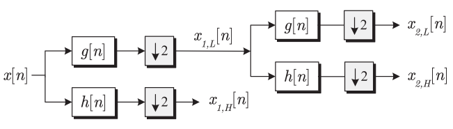
where g[n] is a low pass filter and h[n] is a high pass filter